POLI 144AB Coding Workshop 3
7 minute read
library(tidyverse)
Introduction
Linear regression is a fundamental statistical method used to model the relationship between a dependent variable and one or more independent variables. In this lesson, we will cover the basics of linear regression, including how to implement it in R.
What is Linear Regression?
Linear regression aims to find the best-fitting straight line through the data points, predicting the dependent variable (Y) from the independent variable(s) (X).
Simple Linear Regression
Simple linear regression involves one dependent variable and one independent variable. The model is represented as:
\[Y = \beta_0 + \beta_1X + \epsilon\]- $Y$ is the dependent variable.
- $X$ is the independent variable.
- $\beta_0$ is the intercept.
- $\beta_1$ is the slope of the line.
- $\epsilon$ is the error term.
Dataset
For this lesson, we’ll use the mtcars dataset available in R.
# Load the dataset
data(mtcars)
force(mtcars)
##                      mpg cyl  disp  hp drat    wt  qsec vs am gear carb
## Mazda RX4           21.0   6 160.0 110 3.90 2.620 16.46  0  1    4    4
## Mazda RX4 Wag       21.0   6 160.0 110 3.90 2.875 17.02  0  1    4    4
## Datsun 710          22.8   4 108.0  93 3.85 2.320 18.61  1  1    4    1
## Hornet 4 Drive      21.4   6 258.0 110 3.08 3.215 19.44  1  0    3    1
## Hornet Sportabout   18.7   8 360.0 175 3.15 3.440 17.02  0  0    3    2
## Valiant             18.1   6 225.0 105 2.76 3.460 20.22  1  0    3    1
## Duster 360          14.3   8 360.0 245 3.21 3.570 15.84  0  0    3    4
## Merc 240D           24.4   4 146.7  62 3.69 3.190 20.00  1  0    4    2
## Merc 230            22.8   4 140.8  95 3.92 3.150 22.90  1  0    4    2
## Merc 280            19.2   6 167.6 123 3.92 3.440 18.30  1  0    4    4
## Merc 280C           17.8   6 167.6 123 3.92 3.440 18.90  1  0    4    4
## Merc 450SE          16.4   8 275.8 180 3.07 4.070 17.40  0  0    3    3
## Merc 450SL          17.3   8 275.8 180 3.07 3.730 17.60  0  0    3    3
## Merc 450SLC         15.2   8 275.8 180 3.07 3.780 18.00  0  0    3    3
## Cadillac Fleetwood  10.4   8 472.0 205 2.93 5.250 17.98  0  0    3    4
## Lincoln Continental 10.4   8 460.0 215 3.00 5.424 17.82  0  0    3    4
## Chrysler Imperial   14.7   8 440.0 230 3.23 5.345 17.42  0  0    3    4
## Fiat 128            32.4   4  78.7  66 4.08 2.200 19.47  1  1    4    1
## Honda Civic         30.4   4  75.7  52 4.93 1.615 18.52  1  1    4    2
## Toyota Corolla      33.9   4  71.1  65 4.22 1.835 19.90  1  1    4    1
## Toyota Corona       21.5   4 120.1  97 3.70 2.465 20.01  1  0    3    1
## Dodge Challenger    15.5   8 318.0 150 2.76 3.520 16.87  0  0    3    2
## AMC Javelin         15.2   8 304.0 150 3.15 3.435 17.30  0  0    3    2
## Camaro Z28          13.3   8 350.0 245 3.73 3.840 15.41  0  0    3    4
## Pontiac Firebird    19.2   8 400.0 175 3.08 3.845 17.05  0  0    3    2
## Fiat X1-9           27.3   4  79.0  66 4.08 1.935 18.90  1  1    4    1
## Porsche 914-2       26.0   4 120.3  91 4.43 2.140 16.70  0  1    5    2
## Lotus Europa        30.4   4  95.1 113 3.77 1.513 16.90  1  1    5    2
## Ford Pantera L      15.8   8 351.0 264 4.22 3.170 14.50  0  1    5    4
## Ferrari Dino        19.7   6 145.0 175 3.62 2.770 15.50  0  1    5    6
## Maserati Bora       15.0   8 301.0 335 3.54 3.570 14.60  0  1    5    8
## Volvo 142E          21.4   4 121.0 109 4.11 2.780 18.60  1  1    4    2
# Build the linear model
# lm(dependent variable ~ independent variable)
model_1 <- lm(mpg ~ wt, data = mtcars)
model_2 <- lm(mpg ~ hp, data = mtcars)

# Summary of the model
summary(model_1)
##
## Call:
## lm(formula = mpg ~ wt, data = mtcars)
##
## Residuals:
##     Min      1Q  Median      3Q     Max
## -4.5432 -2.3647 -0.1252  1.4096  6.8727
##
## Coefficients:
##             Estimate Std. Error t value Pr(>|t|)
## (Intercept)  37.2851     1.8776  19.858  < 2e-16 ***
## wt           -5.3445     0.5591  -9.559 1.29e-10 ***
## ---
## Signif. codes:  0 '***' 0.001 '**' 0.01 '*' 0.05 '.' 0.1 ' ' 1
##
## Residual standard error: 3.046 on 30 degrees of freedom
## Multiple R-squared:  0.7528, Adjusted R-squared:  0.7446
## F-statistic: 91.38 on 1 and 30 DF,  p-value: 1.294e-10
summary(model_2)
##
## Call:
## lm(formula = mpg ~ hp, data = mtcars)
##
## Residuals:
##     Min      1Q  Median      3Q     Max
## -5.7121 -2.1122 -0.8854  1.5819  8.2360
##
## Coefficients:
##             Estimate Std. Error t value Pr(>|t|)
## (Intercept) 30.09886    1.63392  18.421  < 2e-16 ***
## hp          -0.06823    0.01012  -6.742 1.79e-07 ***
## ---
## Signif. codes:  0 '***' 0.001 '**' 0.01 '*' 0.05 '.' 0.1 ' ' 1
##
## Residual standard error: 3.863 on 30 degrees of freedom
## Multiple R-squared:  0.6024, Adjusted R-squared:  0.5892
## F-statistic: 45.46 on 1 and 30 DF,  p-value: 1.788e-07
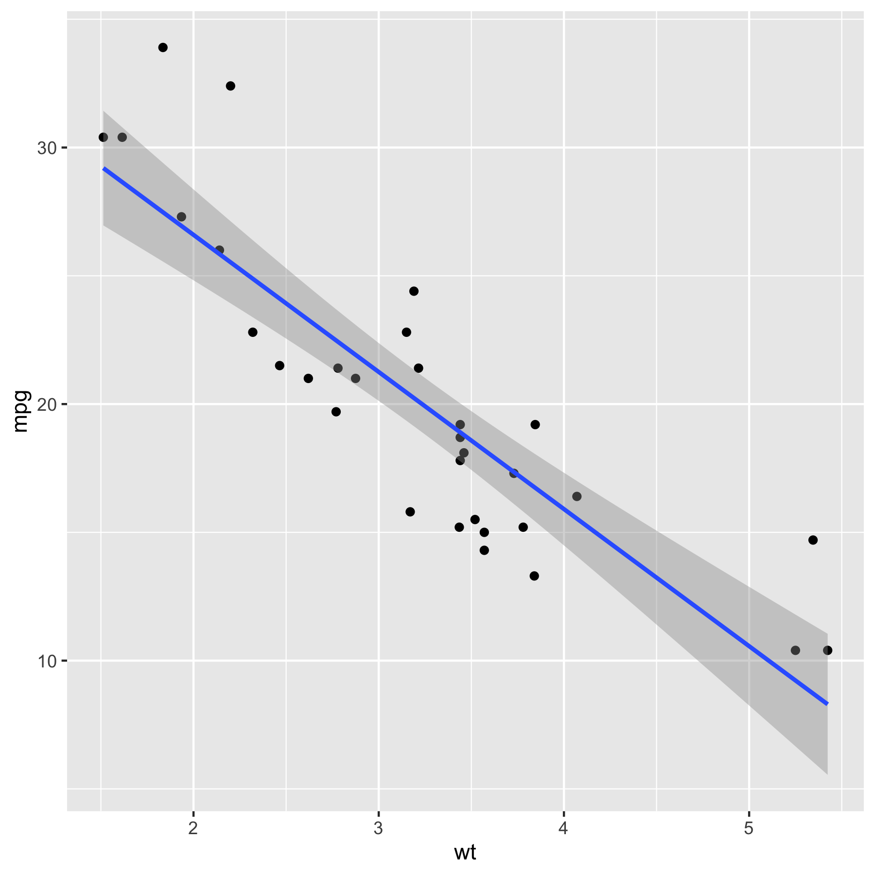
# Plotting the data points
mtcars %>%
  ggplot(aes(x = wt, y = mpg)) +
  geom_point() +
  geom_smooth(method = "lm", se = T)
# Build the multiple linear regression model
model_mult <- lm(mpg ~ wt + hp, data = mtcars)

# Summary of the model
summary(model_mult)
##
## Call:
## lm(formula = mpg ~ wt + hp, data = mtcars)
##
## Residuals:
##    Min     1Q Median     3Q    Max
## -3.941 -1.600 -0.182  1.050  5.854
##
## Coefficients:
##             Estimate Std. Error t value Pr(>|t|)
## (Intercept) 37.22727    1.59879  23.285  < 2e-16 ***
## wt          -3.87783    0.63273  -6.129 1.12e-06 ***
## hp          -0.03177    0.00903  -3.519  0.00145 **
## ---
## Signif. codes:  0 '***' 0.001 '**' 0.01 '*' 0.05 '.' 0.1 ' ' 1
##
## Residual standard error: 2.593 on 29 degrees of freedom
## Multiple R-squared:  0.8268, Adjusted R-squared:  0.8148
## F-statistic: 69.21 on 2 and 29 DF,  p-value: 9.109e-12
A one unit increase in HP (horse power) is correlated with 0.03177 units lower in mile per gallon and is statistically significant at < 0.001 level. A one unit increase in WT (weight) is correlated with 3.877 units lower in mile per gallon and is statistically significant at 0.001 level.
Generating Predictions
After building a linear regression model, we can use it to make predictions. We’ll cover how to generate predictions for both the simple (bivariate) and multiple (multivariate) linear regression models.
Predictions with Simple Linear Regression
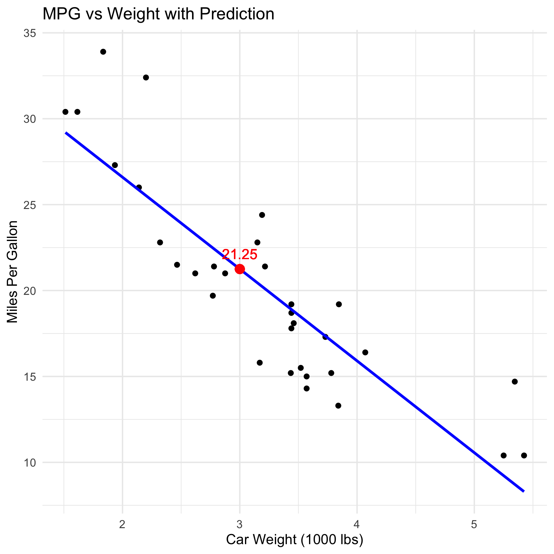
Using the model we created earlier (predicting mpg based on wt), let’s predict the mpg for a car that weighs 3,000 lbs.
new_data <- data.frame(wt = 3)

# Generate prediction

predicted_mpg <- predict(model_1, newdata = new_data)

# Output the prediction

predicted_mpg
##        1
## 21.25171
ggplot(mtcars, aes(x = wt, y = mpg)) +
  geom_point() +
  geom_smooth(method = "lm", col = "blue", se = FALSE) +
  geom_point(aes(x = new_data$wt, y = predicted_mpg), color = "red", size = 3) +
  geom_text(aes(x = new_data$wt, y = predicted_mpg, label = round(predicted_mpg, 2)),
            vjust = -1, color = "red") +
  labs(title = "MPG vs Weight with Prediction",
       x = "Car Weight (1000 lbs)",
       y = "Miles Per Gallon") +
  theme_minimal()