POLI 144AB Coding Workshop 4
6 minute read
Load Shape Data
# install sf to make maps
# install.packages("sf")

library(sf)
library(tidyverse)
library(here)

state_shape <- st_read(here("../Teaching/SS2_2024_POLI144AB/Data/August15_Data/US States Shape Files", "tl_2012_us_state.shp"))
## Reading layer `tl_2012_us_state' from data source
##   `/Users/ericthai/Library/CloudStorage/Dropbox/Teaching/SS2_2024_POLI144AB/Data/August15_Data/US States Shape Files/tl_2012_us_state.shp'
##   using driver `ESRI Shapefile'
## Simple feature collection with 56 features and 17 fields
## Geometry type: MULTIPOLYGON
## Dimension:     XY
## Bounding box:  xmin: -19951910 ymin: -1643352 xmax: 20021890 ymax: 11554790
## Projected CRS: Popular Visualisation CRS / Mercator
county_shape <- st_read(here("../Teaching/SS2_2024_POLI144AB/Data/August15_Data/US County Shape Files", "cb_2018_us_county_500k.shp"))
## Reading layer `cb_2018_us_county_500k' from data source
##   `/Users/ericthai/Library/CloudStorage/Dropbox/Teaching/SS2_2024_POLI144AB/Data/August15_Data/US County Shape Files/cb_2018_us_county_500k.shp'
##   using driver `ESRI Shapefile'
## Simple feature collection with 3233 features and 9 fields
## Geometry type: MULTIPOLYGON
## Dimension:     XY
## Bounding box:  xmin: -179.1489 ymin: -14.5487 xmax: 179.7785 ymax: 71.36516
## Geodetic CRS:  NAD83
census_pop <- readRDS(here("../Teaching/SS2_2024_POLI144AB/Data/August15_Data", "census_pop_1990_2019_cleaned.rds"))

manufacturing_emp <- readRDS(here("../Teaching/SS2_2024_POLI144AB/Data/August15_Data", "manufacturing_emp.rds"))

president_vote <- read_csv(here("../Teaching/SS2_2024_POLI144AB/Data/August15_Data", "1976-2020-president.csv"))
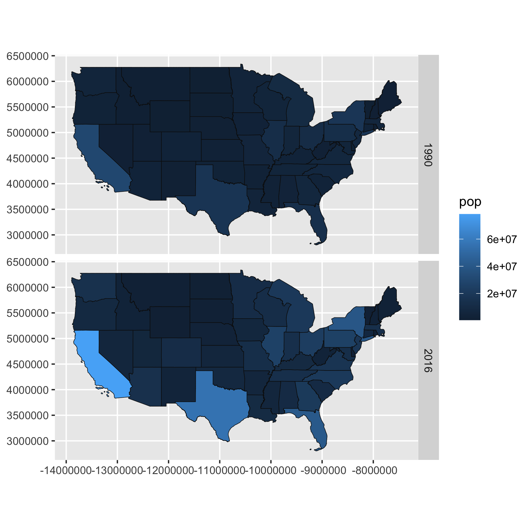
Population 1990 vs 2016
census_pop_cleaned <- census_pop %>%
  group_by(fipstate, year) %>%
  summarise(pop = sum(pop, na.rm=T)) %>%
  ungroup() %>%
  filter(year == 1990 | year == 2016)
census_pop_cleaned %>%
  left_join(state_shape, by=c("fipstate" = "STATEFP")) %>%
  filter(!NAME %in% c("Alaska", "Hawaii"))
## # A tibble: 98 × 20
##    fipstate year       pop OBJECTID REGION DIVISION STATENS  GEOID STUSPS NAME
##    <chr>    <chr>    <dbl>    <int> <chr>  <chr>    <chr>    <chr> <chr>  <chr>
##  1 01       1990   4050055       32 3      6        01779775 01    AL     Alaba…
##  2 01       2016   9727050       32 3      6        01779775 01    AL     Alaba…
##  3 04       1990   3684097       54 4      8        01779777 04    AZ     Arizo…
##  4 04       2016  13882144       54 4      8        01779777 04    AZ     Arizo…
##  5 05       1990   2356586        2 3      7        00068085 05    AR     Arkan…
##  6 05       2016   5979836        2 3      7        00068085 05    AR     Arkan…
##  7 06       1990  29959515       56 4      9        01779778 06    CA     Calif…
##  8 06       2016  78334234       56 4      9        01779778 06    CA     Calif…
##  9 08       1990   3307618       43 4      8        01779779 08    CO     Color…
## 10 08       2016  11078430       43 4      8        01779779 08    CO     Color…
## # ℹ 88 more rows
## # ℹ 10 more variables: LSAD <chr>, MTFCC <chr>, FUNCSTAT <chr>, ALAND <dbl>,
## #   AWATER <dbl>, INTPTLAT <chr>, INTPTLON <chr>, Shape_Leng <dbl>,
## #   Shape_Area <dbl>, geometry <MULTIPOLYGON [m]>
census_pop_cleaned %>%
  left_join(state_shape, by=c("fipstate"="STATEFP")) %>%
  filter(!NAME %in% c("Alaska", "Hawaii")) %>%
  ggplot() +
  geom_sf(aes(geometry = geometry, fill = pop), color = "grey5") +
  facet_grid(rows=vars(year))
# customize!
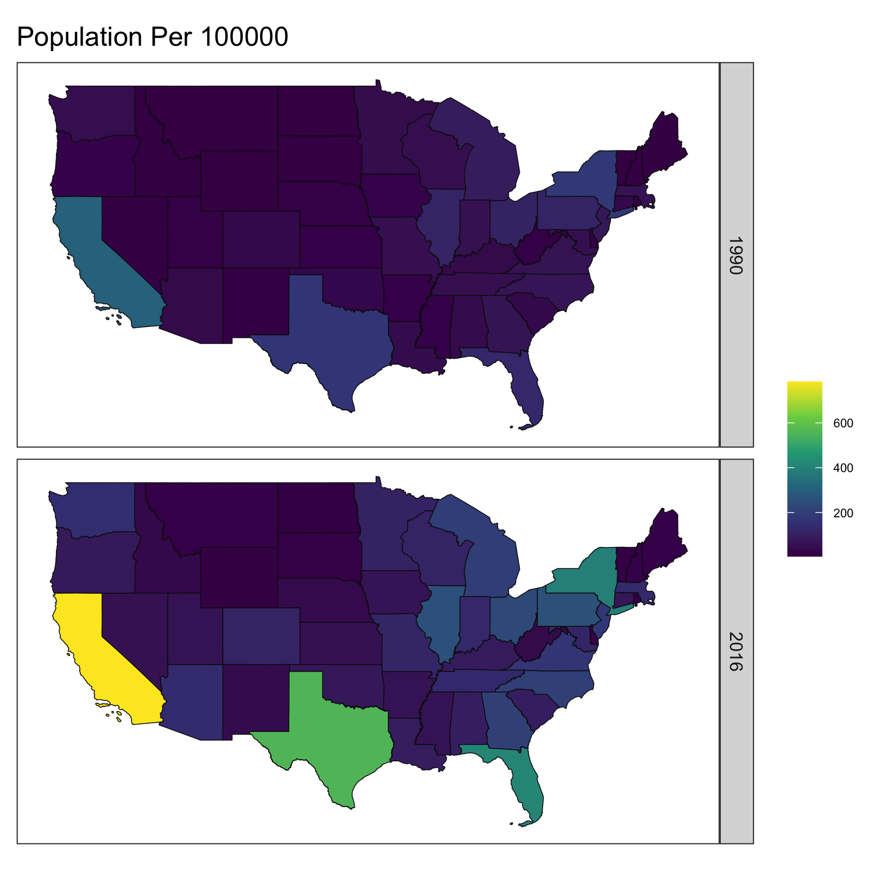
census_pop_cleaned %>%
left_join(state_shape, by=c("fipstate"="STATEFP")) %>%
filter(!NAME %in% c("Alaska", "Hawaii")) %>%
mutate(pop_100000 = pop / 100000) %>%
ggplot() +
geom_sf(aes(geometry = geometry, fill = pop_100000), color = "grey5") +
theme_bw() +
theme(axis.text.x = element_blank(), # Remove x-axis text
axis.text.y = element_blank(), # Remove y-axis text
axis.title.x = element_blank(), # Remove x-axis title
axis.title.y = element_blank(), # Remove y-axis title
axis.ticks = element_blank(), # Remove axis ticks
panel.grid.major = element_blank(), # Remove major grid lines
panel.grid.minor = element_blank(),
legend.text = element_text(size=6)) +
# change the color
scale_fill_viridis_c() +
labs(title = "Population Per 100000",
fill = "") +
facet_grid(rows=vars(year))
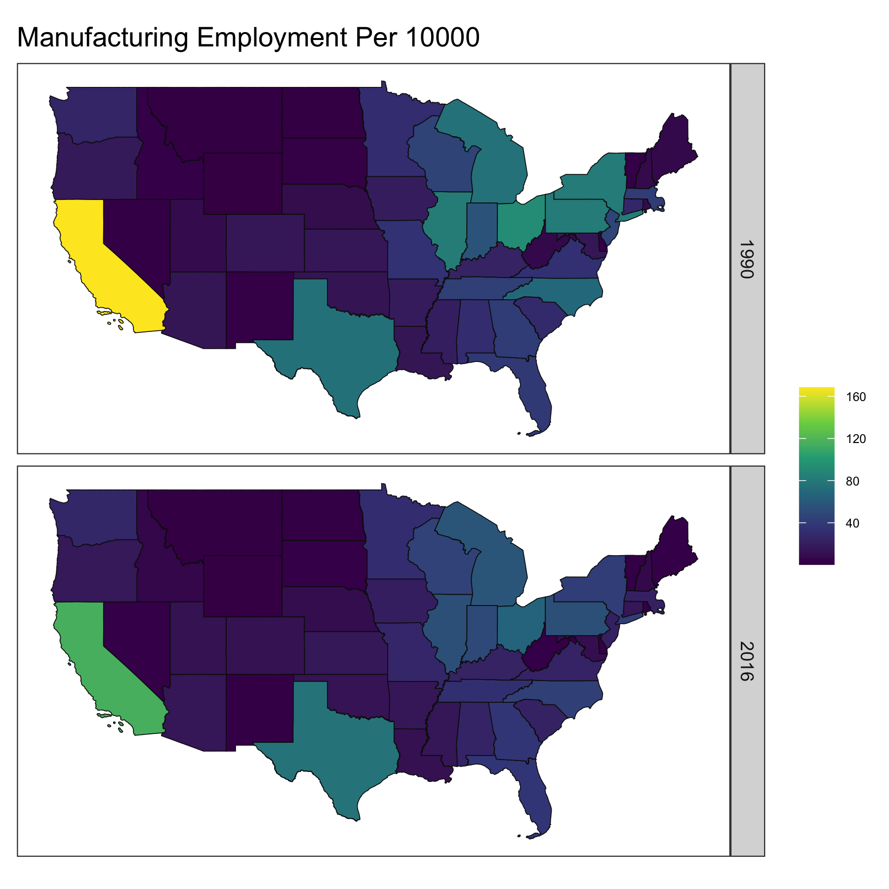
Manufacturing Employment in 1990 vs 2016
# customize!
manufacturing_emp %>%
  left_join(state_shape, by=c("fipstate"="STATEFP")) %>%
  filter(!NAME %in% c("Alaska", "Hawaii")) %>%
  filter(year == 1990 | year == 2016) %>%
  mutate(manufacturing_emp = manufacturing_emp / 10000) %>%
  ggplot() +
  geom_sf(aes(geometry = geometry, fill = manufacturing_emp), color = "grey5") +
  theme_bw() +
  theme(axis.text.x = element_blank(),    # Remove x-axis text
        axis.text.y = element_blank(),    # Remove y-axis text
        axis.title.x = element_blank(),   # Remove x-axis title
        axis.title.y = element_blank(),   # Remove y-axis title
        axis.ticks = element_blank(),     # Remove axis ticks
        panel.grid.major = element_blank(),  # Remove major grid lines
        panel.grid.minor = element_blank(),
        legend.text = element_text(size=6)) +
  # change the color
  scale_fill_viridis_c() +
  labs(title = "Manufacturing Employment Per 10000",
       fill = "") +
  facet_grid(rows=vars(year))
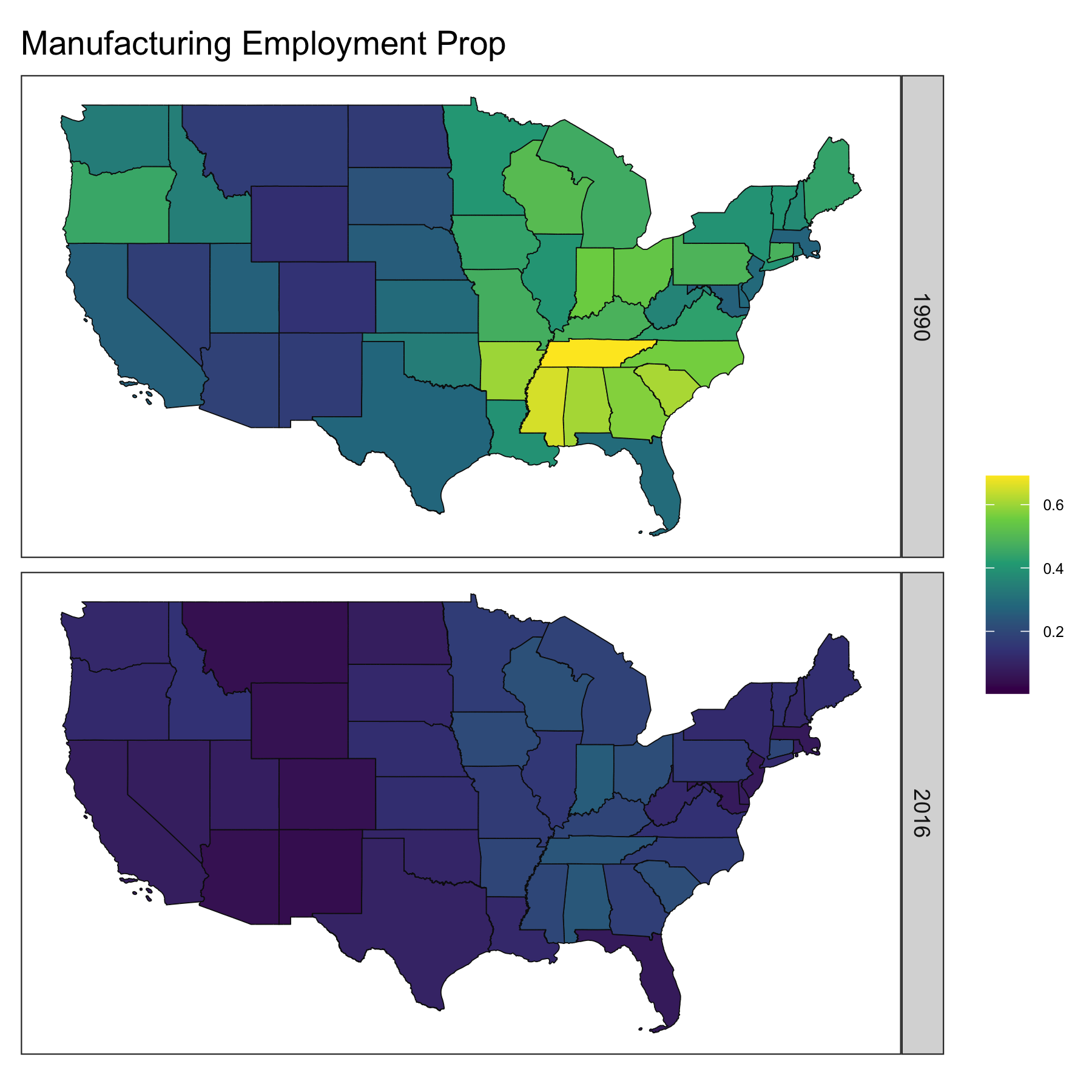
Manufacturing Proportion 1990 vs 2016
# customize!
manufacturing_emp %>%
  left_join(state_shape, by=c("fipstate"="STATEFP")) %>%
  filter(!NAME %in% c("Alaska", "Hawaii")) %>%
  filter(year == 1990 | year == 2016) %>%
  ggplot() +
  geom_sf(aes(geometry = geometry, fill = manufacturing_emp_prop), color = "grey5") +
  theme_bw() +
  theme(axis.text.x = element_blank(),    # Remove x-axis text
        axis.text.y = element_blank(),    # Remove y-axis text
        axis.title.x = element_blank(),   # Remove x-axis title
        axis.title.y = element_blank(),   # Remove y-axis title
        axis.ticks = element_blank(),     # Remove axis ticks
        panel.grid.major = element_blank(),  # Remove major grid lines
        panel.grid.minor = element_blank(),
        legend.text = element_text(size=6)) +
  # change the color
  scale_fill_viridis_c() +
  labs(title = "Manufacturing Employment Prop",
       fill = "") +
  facet_grid(rows=vars(year))
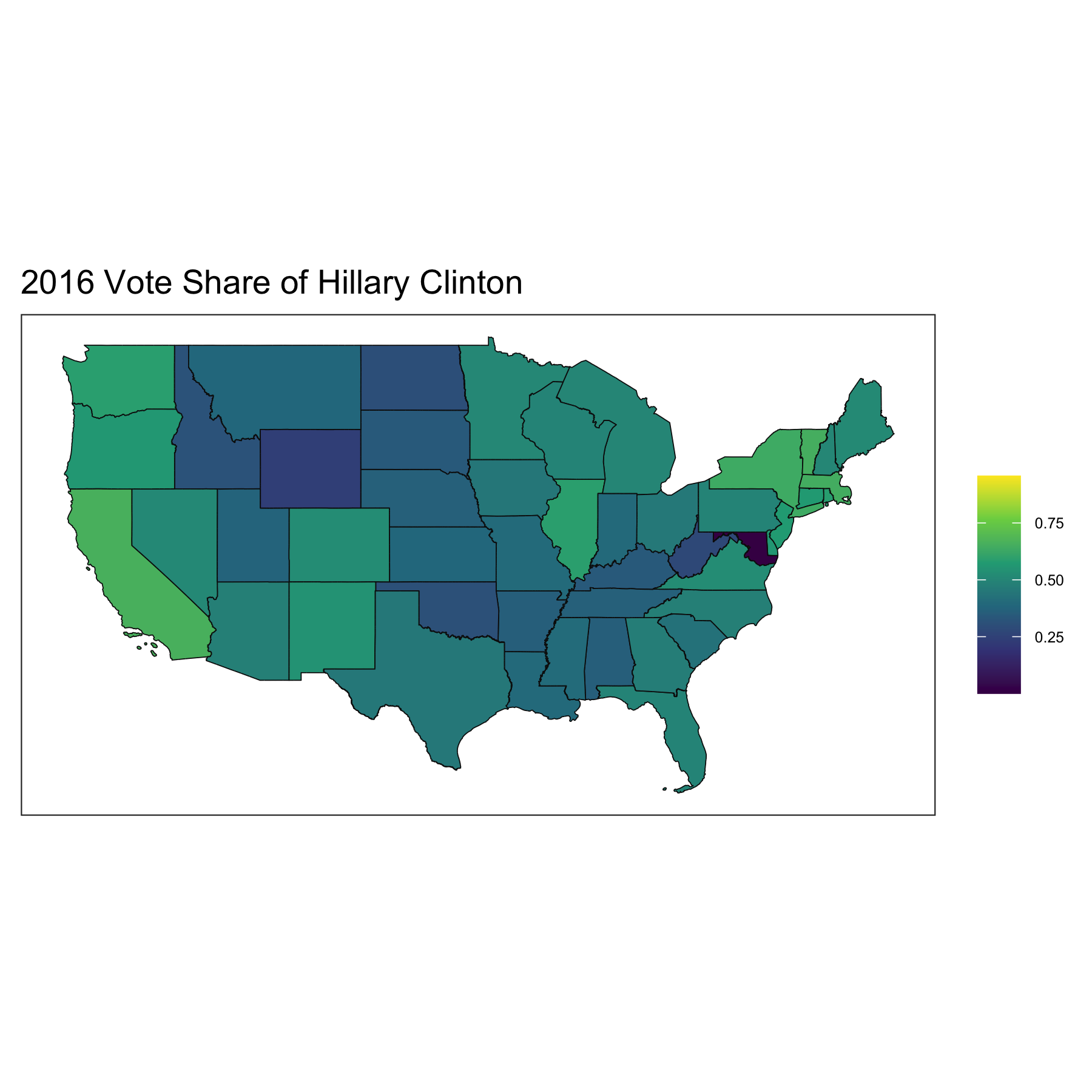
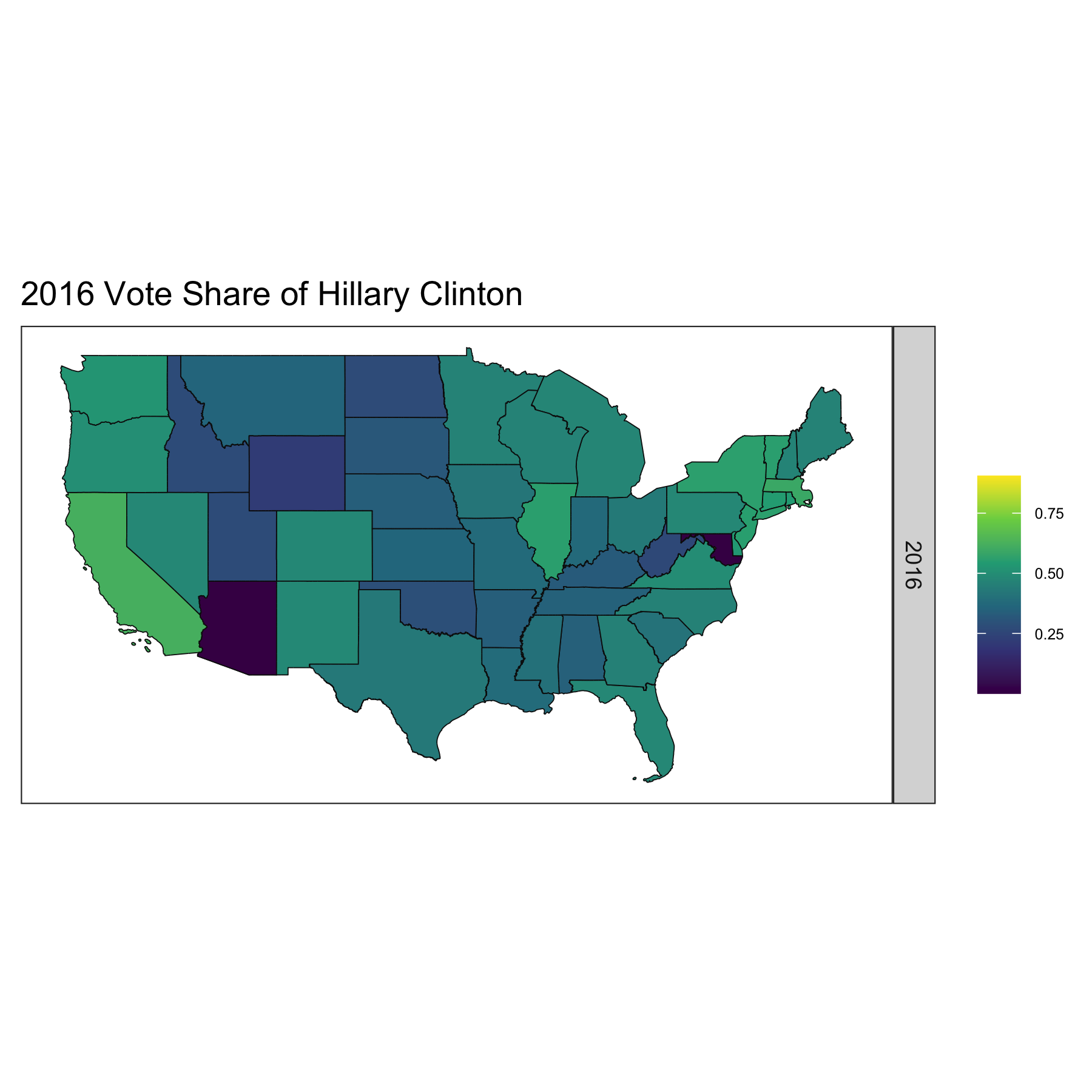
Presidential Election 2016: Hillary Clinton’s Vote Share
president_vote %>%
  # put 0s before 1 digit state_fips to be able to merge
  mutate(fipstate = sprintf("%02d", state_fips)) %>%
  left_join(state_shape, by=c("fipstate"="STATEFP")) %>%
  filter(!NAME %in% c("Alaska", "Hawaii")) %>%
  filter(year == 2016 & party_detailed == "DEMOCRAT") %>%
  mutate(vote_prop = candidatevotes / totalvotes) %>%
  ggplot() +
  geom_sf(aes(geometry = geometry, fill = vote_prop), color = "grey5") +
  theme_bw() +
  theme(axis.text.x = element_blank(),    # Remove x-axis text
        axis.text.y = element_blank(),    # Remove y-axis text
        axis.title.x = element_blank(),   # Remove x-axis title
        axis.title.y = element_blank(),   # Remove y-axis title
        axis.ticks = element_blank(),     # Remove axis ticks
        panel.grid.major = element_blank(),  # Remove major grid lines
        panel.grid.minor = element_blank(),
        legend.text = element_text(size=6)) +
  # change the color
  scale_fill_viridis_c() +
  labs(title = "2016 Vote Share of Hillary Clinton",
       fill = "") +
  facet_grid(rows=vars(year))
president_vote %>%
  filter(year == 2016) %>%
  filter(party_detailed %in% c("REPUBLICAN", "DEMOCRAT")) %>%
  group_by(state) %>%
  mutate(two_party_vote_share = candidatevotes / sum(candidatevotes, na.rm=T)) %>%
  ungroup() %>%
  filter(candidate == "CLINTON, HILLARY") %>%
  mutate(fipstate = sprintf("%02d", state_fips)) %>%
  left_join(state_shape, by=c("fipstate"="STATEFP")) %>%
  filter(!NAME %in% c("Alaska", "Hawaii")) %>%
  ggplot() +
  geom_sf(aes(geometry = geometry, fill = two_party_vote_share), color = "grey5") +
  theme_bw() +
  theme(axis.text.x = element_blank(),    # Remove x-axis text
        axis.text.y = element_blank(),    # Remove y-axis text
        axis.title.x = element_blank(),   # Remove x-axis title
        axis.title.y = element_blank(),   # Remove y-axis title
        axis.ticks = element_blank(),     # Remove axis ticks
        panel.grid.major = element_blank(),  # Remove major grid lines
        panel.grid.minor = element_blank(),
        legend.text = element_text(size=6)) +
  # change the color
  scale_fill_viridis_c() +
  labs(title = "2016 Vote Share of Hillary Clinton",
       fill = "")